TidyTensor is an R package for inspecting and manipulating tensors (multidimensional arrays). i
It provides an improved print() function for summarizing structure, named tensors,
conversion to data frames, and high-level manipulation functions. Designed to complement the
excellent keras package, functionality is layered on top of base R types.
TidyTensor was inspired by a workshop I taught in deep learning with R, and a desire to explain and explore tensors in a more intuitive way.
The github README provides more detail, but
a few samples here won’t hurt. TidyTensors are created with as.tidytensor() or the
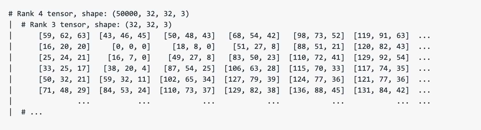
short convenience function tt(). The default print() reveals structure.
library(keras)

images <- dataset_cifar10()$train$x

images %>%
  tt() %>%
  set_ranknames(image, row, col, channel)
# Rank 4 tensor, shape: (50000, 32, 32, 3), ranknames: image, row, col, channel
|  # Rank 3 tensor, shape: (32, 32, 3)
|      [59, 62, 63]  [43, 46, 45]   [50, 48, 43]   [68, 54, 42]   [98, 73, 52]  [119, 91, 63]  ...
|      [16, 20, 20]     [0, 0, 0]     [18, 8, 0]    [51, 27, 8]   [88, 51, 21]  [120, 82, 43]  ...
|      [25, 24, 21]    [16, 7, 0]    [49, 27, 8]   [83, 50, 23]  [110, 72, 41]  [129, 92, 54]  ...
|      [33, 25, 17]   [38, 20, 4]   [87, 54, 25]  [106, 63, 28]  [115, 70, 33]  [117, 74, 35]  ...
|      [50, 32, 21]  [59, 32, 11]  [102, 65, 34]  [127, 79, 39]  [124, 77, 36]  [121, 77, 36]  ...
|      [71, 48, 29]  [84, 53, 24]  [110, 73, 37]  [129, 82, 38]  [136, 88, 45]  [131, 84, 42]  ...
|               ...           ...            ...            ...            ...            ...  ...
|  # ...
TidyTensor can be useful in a variety of ways; here we’ll use k_function() from keras()
to create a function that creates featuremaps:
vgg_model <- application_vgg16(include_top = FALSE, input_shape = c(32, 32, 3))

input <- vgg_model$input
output <- get_layer(vgg_model, name = "block1_conv2")$output

# input shape (N, 32, 32, 3)
# output shape (N, 32, 32, 64) tensor, where last rank are feature maps
compute_featuremaps <- k_function(input, output)
And then visualize the first six featuremaps produced by the first four images:
library(dplyr)

compute_featuremaps(images[1:4, , ,]) %>%
  tt() %>%
  set_ranknames(image, row, col, featuremap) %>%
  as.data.frame(allow_huge = T) %>%
  filter(featuremap <= 6) %>%
  ggplot() +
    geom_tile(aes(x = col, y = row, fill = value)) +
    facet_grid(image ~ featuremap) +
    coord_equal() +
    scale_y_reverse()
