I’ve been studying up on deep learning recently (I know, trendy), and I learned something along the way that I think is just incredible.1
First, a little background: deep learning models are artificial neural networks, represented as potentially thousands of nodes with millions of weighted connections between them. Input numbers are fed in to some nodes on one side, and out pops output numbers from some nodes on the other side, after winding through the nodes and weighted connections. The goal is to adjust the connection weights such that the outputs are what we want for any given input.


More formally, we define a cost function that compares example model outputs to known good outputs (with the cost being higher for incorrect outputs), and minimize the cost by adjusting the weights. Gradient descent is a very popular method employed for this process.
To make matters easy, let’s suppose there are just 2 weights, such that the cost function for a given input and output looks like so:

A given set of weights exists on this surface as a point with a corresponding cost–maybe just this side of that big peak. The gradient is the direction that slopes most upward (opposite the direction a ball placed on that point would start to roll). If we know the gradient, we know how we should tweak the weights to lower our cost efficiently. Gradient descent is to iterate this process a number of times until the gradient is zero (which may not be the lowest overall cost, if we fall into a local minimum like the left pit above).
Anyway, gradient descent is all about derivatives: the gradient in the direction of the first weight \(w_1\) is the partial derivative of the cost function \(f\) with respect to that weight, \(\frac{d}{dw_1}f\). In real deep learning models, this means differentiating a function of thousands or millions of variables, where the function itself is incredibly complex due to all that neural-networky stuff.
Computational differentation
For what follows, We’re going to consider only functions of a single variable, \(\mathbb{R} \rightarrow \mathbb{R}\).

So, how do we get a computer to differentiate a function? Sure, we can query for the cost value at any particular point. How can we tell what the slope is near there?
Until recently, I only knew of two ways: symbolic differentiation and numerical derivation.
Symbolic differentation
Symbolic differentiation is basic calculus–manipulating function formulas to come up with other function formulas. Some software can do this as well, for example Wolfram Alpha can tell me that the \(\frac{d}{d x}(2 x + 3 x ^ 3)\) is \(2 + 9 x ^2\). This is pretty cool in itself, because the computer isn’t executing this code (it’s not multiplying any actual number by 2), it’s manipulating the formula as data.2
input: D[2 x + 3 x^3, x]
output: 2 + 9 x^2
However, because the functions used in deep learning are so huge and complex, this method isn’t used, as the formulas can grow exponentially in the size of the network.
Numerical differentation
This is the straightforward programming way to compute the derivative of a function at a point \(x\), or at least an approximation of it. Supposing f() is the function, and x = 2, we can evaluate the function at x and nearby:
x <- 2
xnear <- 2.0001
y <- f(x)
ynear <- f(xnear)
slope <- (ynear - y)/(xnear - x)
This doesn’t work well in practice: if xnear is very close to x then roundoff errors come into play, but if xnear is far from x then the approximation isn’t very good.
Automatic differentation
Automatic differentiation exploits the fact that there are only so many “base” functions that computers support (modern CPUs support things like + and *, and now even sqrt() and sin()), and generally these have a well-defined derivative function. Further, rules of calculus specify how to compute derivatives of a complicated function based on derivatives of component functions. For example, if we want to compute \(\frac{d}{dx}(\sin(x) + \cos(x))\), this is \(\frac{d}{dx}\sin(x) + \frac{d}{dx}\cos(x) = \cos(x) - \sin(x)\). (The derivative of \(\sin(x)\) is \(\cos(x)\), and the derivative of \(\cos(x)\) is \(-\sin(x)\).) Thus, by applying derivative rules we eventually get back to known “base” functions with already-defined derivatives.
The compute above is important: if we want to evaluate the derivative at a given x, and we can work with functions in code this way (add them, subtract them, divide them, etc.), then we can actually call those functions. This is the specialty of functional languages, where functions are themselves types of data that can be operated on (as in symbolic differentiation) and called (as in numerical differentiation).
This is a pretty cool idea, so I fired up my favorite functional language, R, and gave it a shot.
f() and f’() pairs
First, we need easy access to a function and its derivative function: they’re a matched set. I first thought to hold these in a small R list, starting with \sin() and \cos(), calling them mysin and mycos.
mycos <- list(f = cos, deriv = sin)
mysin <- list(f = sin, deriv = cos)
This worked to some degree, but to call the function or derivative I needed the awkward syntax mysin$f(x) or mysin$deriv(x). Worse, there’s no obvious way to take a second derivative: mysin$deriv(x) is a function in x, but I can’t get its derivative in an automated way.3
To work around the syntax issue, I made mycos() and mysin() callable functions:
mycos <- function(x) {
  return(cos(x))
}

mysin <- function(x) {
  return(sin(x))
}
Now, how can we attach the derivative of mysin to mysin itself, a function? Fortunately R allows us to assign “attributes” to any type of data, including functions.4 Ideally the derivative of mysin is mycos rather than just cos; this would allow for second derivatives and higher. My first attempt tried to assign the attributes directly.
attr(mycos, "getderiv") <- mysin
attr(mysin, "getderiv") <- mycos
However, order affects became apparent, because <- is assignment-by-copy. When we run attr(mycos, "getderiv") <- mysin it’s attaching a copy of mysin which as of yet doesn’t have a derivative attached, effectively breaking the ability to compute the second derivative of mycos. Then on attr(mysin, "getderiv") <- mycos, the mysin function gets its derivative as a copy of mycos that also has a workable first-level derivative. So for mysin we can get first and second derivatives, but not third. (Tl;dr: it didn’t work.)
Here’s the solution I landed on. In the "getderiv" attribute, we store an anonymous function whose only job is to return the derivative function. After setting the attribute, we can even call it with attr(mycos, "getderiv")() syntax.
attr(mycos, "getderiv") <- function() {return(mysin)}
attr(mysin, "getderiv") <- function() {return(mycos)}
deriv <- attr(mysin, "getderiv")()
print(deriv(c(-1, 0, 1)))
## [1] 0.5403023 1.0000000 0.5403023print(cos(c(-1, 0, 1)))## [1] 0.5403023 1.0000000 0.5403023print(deriv)## function(x) {
## return(cos(x))
## }
## attr(,"getderiv")
## function ()
## {
## return(mysin)
## }Notice that deriv is a function that does indeed return cos(x), and furthermore, it itself has a "getderiv" function! This means we can get its derivative:
deriv_deriv <- attr(deriv, "getderiv")()
print(deriv_deriv(c(-1, 0, 1)))
## [1] -0.841471 0.000000 0.841471print(deriv_deriv)## function(x) {
## return(sin(x))
## }
## attr(,"getderiv")
## function ()
## {
## return(mycos)
## }And we can continue to do so, because each function comes packaged with an anonymous function that returns the derivative. These anonymous functions are also closures: function() {return(mysin)} contains mysin bound to (referencing) the data in the calling scope, not a copy (see Appendix below for details). Note that mysin isn’t evaluated here until the anonymous function is run; otherwise we’d have an infinite-recursion issue.
Calling attr(mycos, "getderiv")() is really clunky, so let’s create a derivative function.
d <- function(f) {
  deriv <- attr(f, "getderiv")()
  return(deriv)
}
This is a higher-order function: it takes a function f (which is a function in x) and returns a function (the derivative). This makes good sense, as that’s what the derivative operator is: a function that maps functions to other functions. To call the derivative, we can now use d(mycos)(x), which is starting to look as much like mathematical notation as code.
x <- c(-1, 0, 1)
print(d(mysin)(x))    # calculate and compute derivative of cosin
## [1] 0.5403023 1.0000000 0.5403023print(cos(x)) # should be the same## [1] 0.5403023 1.0000000 0.5403023We can even do multiple derivatives:
x <- c(-1, 0, 1)
print(d(d(mycos))(x))    # calculate and compute 2nd derivative of cosin
## [1] 0.5403023 1.0000000 0.5403023print(mycos(x)) # should be the same## [1] 0.5403023 1.0000000 0.5403023Let’s see if we can plot mysin(x) and d(mysin)(x) for a sanity check.
library(ggplot2)
library(tidyr)

# create columns based on function and derivative values
xs <- seq(0, 3*pi, 0.1)
df <- data.frame(x = xs,
                 fx = mysin(xs),
                 dfx = d(mysin)(xs))

# reshape for plotting
df_toplot <- gather(df, ytype, value, -x)

p <- ggplot() +
  geom_line(data = df_toplot, aes(x = x, y = value, color = ytype))
plot(p)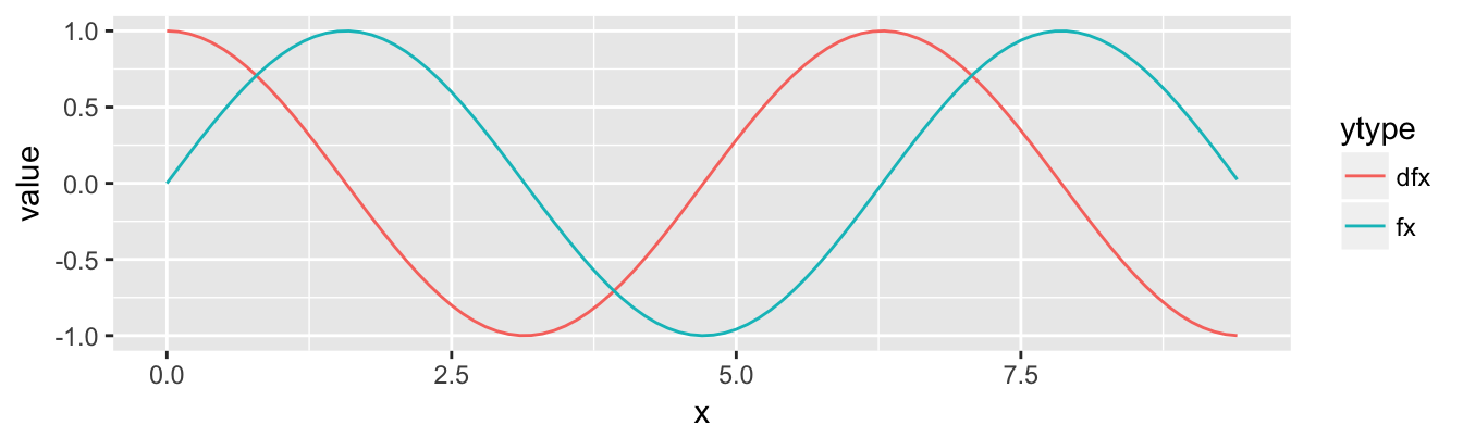
So cool.
Addition and Subtraction
Now that we’ve got the representation worked out, let’s try implementing addition of functions, and derivatives of additions. Mathematically, we want to represent \(\frac{d}{dx}(f(x) + g(x)) = \frac{d}{dx}f(x) + \frac{d}{dx}g(x)\). Here \(+\) is also acting as a higher-order function, taking two input functions \(f\) and \(g\) and returning the addition. It’s an “infix” function, with the function name in the middle of the two parameters.
R lets us create infix functions easily, by using % in the function name. If `%add%` <- function(a, b) { return(a + b)}, then we can call either `%add%`(2, 5) or 2 %add% 5 to get back 7. We just have to use the backticks when defining or using prefix notation.
Let’s define a %+% function for our functions. As above the result of %+% should also come paired with its derivative, the sum of the functions run through d().
`%+%` <- function(f, g) {
  func <- function(x) {
    return(f(x) + g(x))
  }

  attr(func, "getderiv") <- function() {return(d(f) %+% d(g))}
  return(func)
}
Some interesting stuff is happening here: true to form, %+% is a function mapping two input functions in x to a single output function in x. Defined inside, func calls the input functions on the given x (and these are bound via closure). Like mycos and mysin above, the "getderiv" attribute is a function that returns the derivative, and since we create that derivative via d() and the %+% operator, it will also have its own derivative attached. (We’re working now on the assumption that all higher-order functions we create will take and return such matched-pair functions.) Finally, just as above, d(f) %+% d(g) is not evaluated, just defined with variables bound, so there’s no infinite recursion. Basically a lazy list of functions.5
Let’s try it.
print(sin(0.5))## [1] 0.4794255print(cos(0.5))## [1] 0.8775826print(sin(0.5) + cos(0.5))## [1] 1.357008sumfunc <- mysin %+% mycos
print(sumfunc(0.5))## [1] 1.357008print(cos(0.5) + cos(0.5))## [1] 1.755165sumfunc <- mycos %+% d(mysin) # cos + cos
print(sumfunc(0.5))## [1] 1.755165A plot:
xs <- seq(0, 3*pi, 0.1)
df <- data.frame(x = xs,
                 fx = mycos(xs),
                 gx = mysin(xs),
                 sumfxgx = (mycos %+% mysin)(xs))

df_toplot <- gather(df, ytype, value, -x)

p <- ggplot() +
  geom_line(data = df_toplot, aes(x = x, y = value, color = ytype))
plot(p)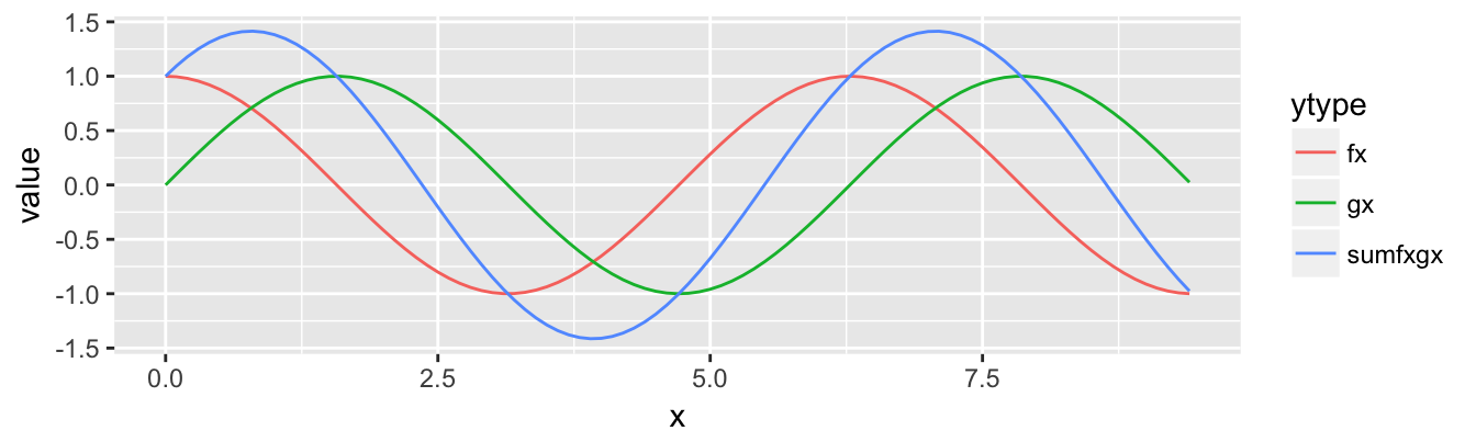
Let’s get %-% out of the way while we’re at it.
`%-%` <- function(f, g) {
  func <- function(x) {
    return(f(x) - g(x))
  }

  attr(func, "getderiv") <- function() {return(d(f) %-% d(g))}
  return(func)
}
Multiplication and Division
Now it’s time to get brave, and implement %*% with the product rule, \(\frac{d}{dx}(f(x) g(x)) = g(x)\frac{d}{dx}f(x) + f(x)\frac{d}{dx}g(x)\), or more succinctly \((f \cdot g)' = f'\cdot g + g'\cdot f\). In this case the derivative uses all four of d(f), f, d(g) and g.
`%*%` <- function(f, g) {
  func <- function(x) {
    return(f(x) * g(x))
  }

  attr(func, "getderiv") <- function() {return((g %*% d(f)) %+% (f %*% d(g)))}
  return(func)
}
Crossing fingers…
xs <- seq(0, 3*pi, 0.1)
df <- data.frame(x = xs,
                 fx = mysin(xs),
                 gx = mycos(xs),
                 fxgx = (mycos %*% mysin)(xs))

df_toplot <- gather(df, ytype, value, -x)

p <- ggplot() +
  geom_line(data = df_toplot, aes(x = x, y = value, color = ytype))
plot(p)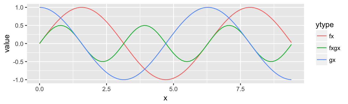
And %/%, based on \((f/g)' = (f' g - g'f)/(g^2)\).
`%/%` <- function(f, g) {
  func <- function(x) {
    return(f(x)/g(x))
  }

  attr(func, "getderiv") <- function() {return( ((d(f) %*% g) %-% (d(g) %*% f)) %/% (g %*% g) )}
  return(func)
}
Constants and Variables
Now, given that we can handle multiplication, can we compute \(\frac{d}{dx}2x\) and get back just 2, or do we need a special case? It turns out we can use our %*% function, if we can treat 2 as a function. Specifically, we want it to be a function in x that always returns 2, no matter the input, since this will allow us to properly combine it with the others.
It will also need an attached derivative. The derivative of a constant is 0, also a constant, which we’ll represent in the same way. Let’s create a const() that returns such a function given the constant of interest; thus const(2) would return one of our functions, as would const(0).
const <- function(input) {
  func <- function(x) {
    return(input)
  }

  attr(func, "getderiv") <- function() { return(const(0)) }
  return(func)
}
Here again closures playing an integral role.6 I also like that a const() function’s derivative is just const(0), and d() maps const(0) to itself.
xs <- seq(0, 3*pi, 0.1)
df <- data.frame(x = xs,
                 fx = (mysin %+% const(2))(xs),
                 dfx = d(mysin %+% const(2))(xs))

df_toplot <- gather(df, ytype, value, -x)

p <- ggplot() +
  geom_line(data = df_toplot, aes(x = x, y = value, color = ytype))
plot(p)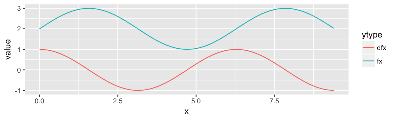
By the way, footnote readers know that we made a mistake in the definition of mycos earlier, in that d(mycos) should be const(-1) %*% mysin rather than just mysin. Now that we can work with constants like -1 we can finally fix it:
attr(mycos, "getderiv") <- function() {return(const(-1) %*% mysin)}We still can’t quite compute \(\frac{d}{dx}2x\) because we don’t yet have a way to represent \(x\); all we have to work with are functions, and now constants (as functions). Much like our const() function though, we can treat \(x\) like a function: one that just returns its input, with a derivative of const(1).
xvar <- function(x) {
  return(x)
}

attr(xvar, "getderiv") <- function() {return(const(1))}
Now we can refer to the \(x\) variable as a function by xvar:
xs <- seq(0, 3*pi, 0.1)
df <- data.frame(x = xs,
                 fx = (const(2) %*% xvar)(xs),
                 dfx = d(const(2) %*% xvar)(xs))

df_toplot <- gather(df, ytype, value, -x)

p <- ggplot() +
  geom_line(data = df_toplot, aes(x = x, y = value, color = ytype))
plot(p)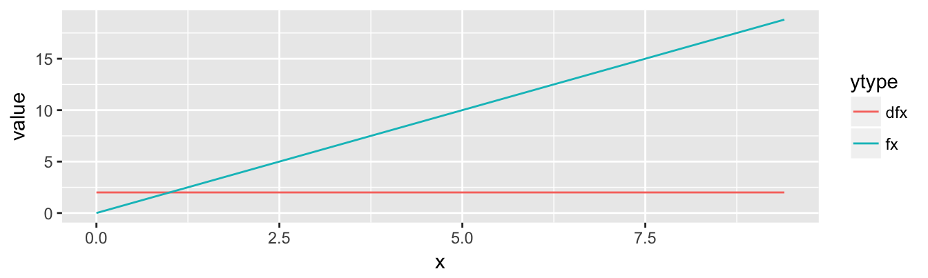
Composition
What about something like \(\frac{d}{dx}\sin(\cos(x))\)? Mathematically this is derived with the chain rule \(\frac{d}{dx}f(g(x)) = f'(g(x))g'(x)\). But \(\sin(\cos(x))\) is difficult to represent in our scheme, since mysin(mycos) would nonsensically attempt to call mysin on the mycos function. What we need is the composition operator, \(\circ\), which is the infix version of calling \(f\) on the result of \(g\): \((f \circ g)(x) = f(g(x))\). We’ll use %o%:
`%o%` <- function(f, g) {
func <- function(x) {
return(f(g(x)))
}
attr(func, "getderiv") <- function() {return( (d(f) %o% g) %*% d(g) )}
return(func)
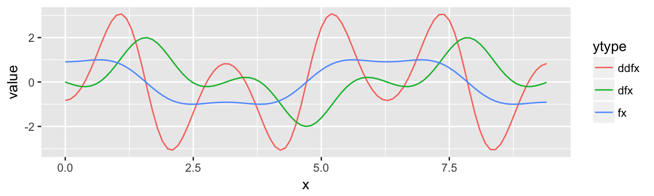
}Let’s have fun with \(\sin(2\cos(x))\) and its first and second derivatives.
xs <- seq(0, 3*pi, 0.1)
df <- data.frame(x = xs,
                 fx = (mysin %o% (const(2) %*% mycos))(xs),
                 dfx = d(mysin %o% (const(2) %*% mycos))(xs),
                 ddfx = d(d(mysin %o% (const(2) %*% mycos)))(xs))

df_toplot <- gather(df, ytype, value, -x)

p <- ggplot() +
  geom_line(data = df_toplot, aes(x = x, y = value, color = ytype))
plot(p)
Power Rules
Rather than implement the power rule, \(\frac{d}{dx}x^n = nx^{n-1}\), or even the general power rule, \(\frac{d}{dx}f(x)^n = nf(x)^{n-1}\frac{d}{dx}f(x)\), we’ll go straight for the functional generalized power rule: \((f^g)' = -f^g\left( f' \frac{g}{f} + g' \ln f \right)\). This version derivates a function raised to the power of another, as in \(\frac{d}{dx}\cos(x)^{\sin(s)}\).
First though, we need to implement the natural logarithm, whose derivative is \(\frac{d}{dx}\ln(x) = 1/x\). (R uses log() for natural logarithm.)
myln <- function(x) {
  return(log(x))
}
attr(myln, "getderiv") <- function() {return(const(1) %/% xvar)}


`%^%` <- function(g, h) {
  func <- function(x) {
    return(g(x) ^ h(x))
  }

  attr(func, "getderiv") <- function() {return(
                                           const(-1) %*% (g %^% h) %*%
                                                   (
                                                     (d(h) %*% (myln %o% g)) %+%
                                                     (h %*% (d(g) %/% g))
                                                   )
                                              )}
  return(func)
}
This example only plots \(\cos^3(x)\) and \(\frac{d}{dx}\cos^3(x)\), but since const(3) is a function in x it fits in this scheme too.
xs <- seq(0, 3*pi, 0.1)
df <- data.frame(x = xs,
                 fx = (mycos %^% const(3))(xs),
                 dfx = d(mycos %^% const(3))(xs))
## Warning in log(x): NaNs produceddf_toplot <- gather(df, ytype, value, -x)
p <- ggplot() +
geom_line(data = df_toplot, aes(x = x, y = value, color = ytype))
plot(p)## Warning: Removed 16 rows containing missing values (geom_path).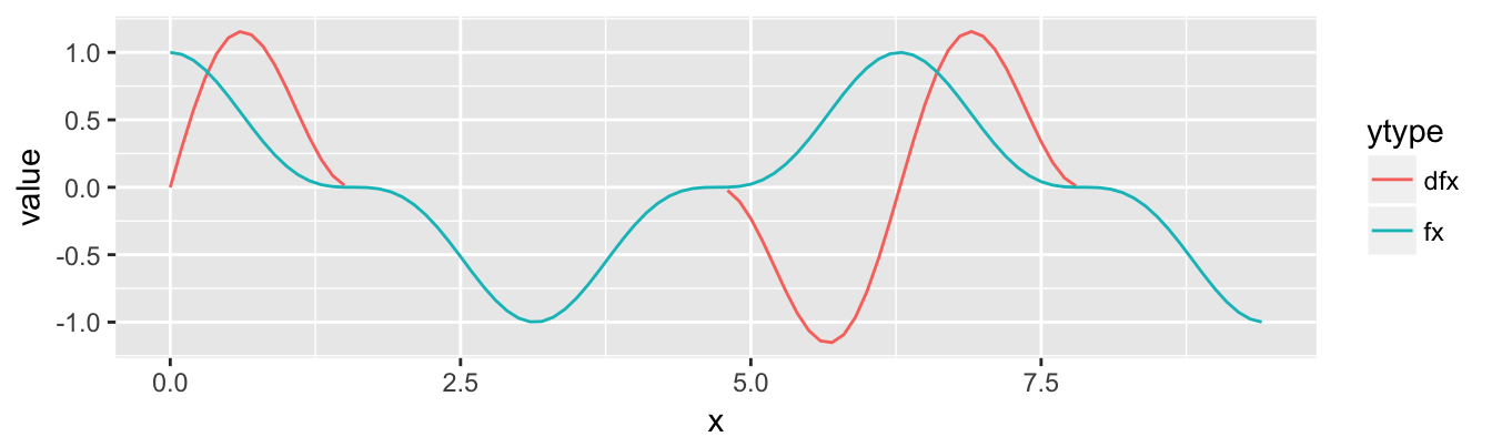
When \(f(x)\) is negative the derivative isn’t defined according to the generalized power rule, because the logarithm isn’t defined for negative numbers. The general power rule would work, but can only accept a const() as the power.
Speaking of logarithms and exponents, here’s \(e^x\), which is its own derivative:
# this one is too dang easy ;)
myexp <- function(x) {
  return(exp(x))
}
attr(myexp, "getderiv") <- function() {return(myexp)}
Efficiency
By my understanding, there are two types of automatic differentiation. The first, forward accumulation, is what we’ve implemented: derivatives are computed for functions in terms of their component functions, recursively. In the second method, reverse accumulation, derivatives of basic elements are computed, and used & re-used for computing derivatives of their more complex parents.7
Reverse mode has two primary advantages: first, that it is inherently vectorized in cases where the function is of multiple variables such as \(f(x,y) = x + y\), computing the gradient vector \(\left<\frac{d}{dx}f, \frac{d}{dy}f\right>\) in one “pass”. Forward mode can only compute one partial derivative \(\frac{d}{dx}f\) or \(\frac{d}{dy}f\) in a single pass. (We haven’t needed to do this, working solely with functions of one variable.) The second advantage of reverse mode is that derivatives of functions are re-used if they are useful for multiple functions needing them.
I’m not sure what could be done about the first disadvantage of forward mode, but perhaps we can do something about the second. Consider computing a complex expression for a particular value:
f <- ((mycos %*% mysin) %+% (mycos %*% mysin)) %/%
     ((mycos %*% mysin) %+% (mycos %*% mysin))
print(f(1.5))
## [1] 1When this function is called, it recursively computes the component pieces. We can see this more directly if we add lines like print("called %+%") inside of %+% et al, and then run print(f(1.5)). I’ve indented the lines to show the nesting:
## [1] "called %/%"
    ## [1] "called %+%"
        ## [1] "called %*%"
            ## [1] "called mycos"
            ## [1] "called mysin"
        ## [1] "called %*%"
            ## [1] "called mycos"
            ## [1] "called mysin"
    ## [1] "called %+%"
        ## [1] "called %*%"
            ## [1] "called mycos"
            ## [1] "called mysin"
        ## [1] "called %*%"
            ## [1] "called mycos"
            ## [1] "called mysin"
## [1] 1
This example is setup for repeated computation: mycos %*% mysin is computed four times total, twice within the first %+% and twice within the second %+%. Computing d(f)(1.5) required 72 calls! A technique called memoization caches the results of function calls; before a function is called the cache is checked to see if the result has already been computed. The memoise package allows us to easily cache results for our functions by wrapping them in memoise( ).
library(memoise)

`%+%` <- memoise(
  function(f, g) {
    print("called %+%")
    func <- function(x) {
      return(f(x) + g(x))
    }

    attr(func, "getderiv") <- function() {return(d(f) %+% d(g))}
    return(func)
  }
)
The result is that identical sub-functions are reused. Once the need for something like mycos %*% mysin arises, the cache is consulted before the function is called. If the answer is present in the cache, it is used and the function is never called. Here’s the result of print(f(1.5)):
## [1] "called %*%"
## [1] "called %+%"
## [1] "called %/%"
## [1] "called mycos"
## [1] "called mysin"
## [1] 1
The derivative d(f)(1.5) is down to 23 calls from 72.
Summary
Automatic differentiation is a really interesting technique, and it highlights some of the unique features of functional programming. So many operations in mathematics are higher-order functions–I suppose it’s no surprise that lisp (the basis for scheme, which inspired R) was based on the lambda calculus, developed by mathematician Alonzo Church in the 1930’s.
There’s still a lot left to explore, such as functions of multiple variables, gradients (series of partial derivatives), and gradient-descent. Perhaps I’ll be able to cover those in another post.
Some interesting links for those wishing to learn more:
Forward and reverse differentiation, with some example code in Rust and Python: http://www.columbia.edu/~ahd2125/post/2015/12/5/
Another article with code examples, also Rust and Python: https://rufflewind.com/2016-12-30/reverse-mode-automatic-differentiation The tape-based implementation near the end is interesting.
A recent article on a novel, simpler method for automatic differentiation with an implementation library in Haskell: https://arxiv.org/pdf/1804.00746.pdf. This project has been pretty difficult to debug, with all the recursive anonymous functions, lazy evaluation, and especially the untyped nature of R. I can easily see how a rich type system such Haskell’s would be helpful.
Appendix
A quick note on closures: closures are functions that make use of non-local data. Often these are found as “global variables” that should be passed as parameters to the function to make it more portable.
c <- 36

add <- function(x, y) {
  sum <- x + y + c       # x and y are local variables, but c is global
  return(sum)            # ...gross
}

print(add(100, 200))     # prints 336
Interestingly, variables scopes can be nested:
a <- 100            # a is available globally, and to get_inner_func and inner_func

get_inner_func <- function() {
  b <- 200 + a      # b is available to get_inner_func and inner_func

  inner_func <- function() {
    c <- 300 + b    # c is available to inner_func
    return(c)
  }

  return(inner_func)
}

inner_func <- get_inner_func()
inner_func()
What’s more, closures “carry with them” the scope (or environment) they were defined in. So in the above, the function returned by get_inner_func() has it’s own local c, as well as still access to b and a. While accessing variables outside a function’s scope can be risky (they get very hard to debug), it is occasionally very useful as we see here.
There are a couples ways to do closures though: is the environment carried with the function a static snapshot, or subject to change as other functions modify the underlying data? The former is sometimes called ‘close-by-value’ or ‘capture-by-value,’ and the latter sometimes called ‘close-by-reference’ or ‘capture-by-reference.’ R is capture-by-reference. (As some may know, R environments provide one of the few options for reference mechanics in the language.)
Here’s a quick verification of R’s close-by-reference nature, based on this Quora answer. Here a is in the scope of make_inc_get(), while inc_a() and get_a() both use it. In inc_a we use the <<- assignment operator, which assigns “up” the scope hierarchy to the first match, whereas <- creates a local variable.
make_inc_get <- function() {
  a <- 0;

  inc_a <- function() {
    a <<- a + 1
  }

  get_a <- function() {
    return(a)
  }

  return(list(inc_a = inc_a, get_a = get_a))
}

inc_get <- make_inc_get()
inc_get$inc_a()
print(inc_get$get_a())
## [1] 1inc_get$inc_a()
print(inc_get$get_a())## [1] 2inc_get$inc_a()
print(inc_get$get_a())## [1] 3I should note that I’m not an expert in any of these topics–just an enthusiast 😁 The automatic differention here I’m sure bears little resemblance to real engines such as TensorFlow.↩
… as far as I know. The Structure and Interpretation of Computer Languages (SICP) explores this.↩
You may also notice I’ve made a mistake, because the derivative of \(\cos(x)\) should be \(-\sin(x)\), not \(\sin(x)\). However, for the sake of exposition, I’m going to leave it for now: we don’t yet have a clear way to define the negation of a function.
-1 * sinwon’t work, as*isn’t defined for a number and a function.↩JavaScript also allows properties on functions since functions are objects. I think most of this would work very similarly in JavaScript.↩
This took me a while to figure out. Initially I was defining
deriv <- function(x) {return(d(f)(x) + d(g)(x))}, and thenattr(func, "getderiv") <- function() {return(deriv)}. This only allows the first derivative however, becausederivisn’t itself a matched-pair function.↩Sorry, that joke is a little derivative.↩
A more useful overview with code examples can be found here.↩